1.7 Interpreting Motion through Graphs, Formulas, and Data
Three Mystery Motions
Here are three descriptions of motion. Your job: decide whether these describe the same motion or three different motions.
Motion A -- A graph:
[Image: A position-time graph. The curve starts at $x = 0$ at $t = 0$, rises steeply and nearly linearly to about $x = 4\,\text{m}$ at $t = 2\,\text{s}$, then curves and flattens between $t = 2\,\text{s}$ and $t = 4\,\text{s}$ reaching $x = 6\,\text{m}$, then resumes rising more steeply from $t = 4\,\text{s}$ onward.]
Motion B -- A data table:
| $t$ (s) | $x$ (m) |
|---|---|
| 0.0 | 0.00 |
| 0.5 | 0.88 |
| 1.0 | 2.00 |
| 1.5 | 3.13 |
| 2.0 | 4.00 |
| 2.5 | 4.63 |
| 3.0 | 5.00 |
| 3.5 | 5.38 |
| 4.0 | 6.00 |
| 4.5 | 7.13 |
| 5.0 | 9.00 |
Motion C -- An equation:
$$x(t) = \frac{1}{3}t^3 - 2t^2 + 4t$$
Before reading on: Look at all three carefully. Are these describing the same motion, or three different motions? What evidence supports your answer?
Take a moment. Compare values. Check a point or two from the table against the equation. Eyeball the graph's shape against what the equation predicts.
They are the same motion, seen through three different lenses. The graph shows you the shape at a glance. The table gives you precise sampled values. The equation gives you a compact rule that generates every point. Three representations, one reality.
This is what this section -- and in many ways, this entire chapter -- is about.
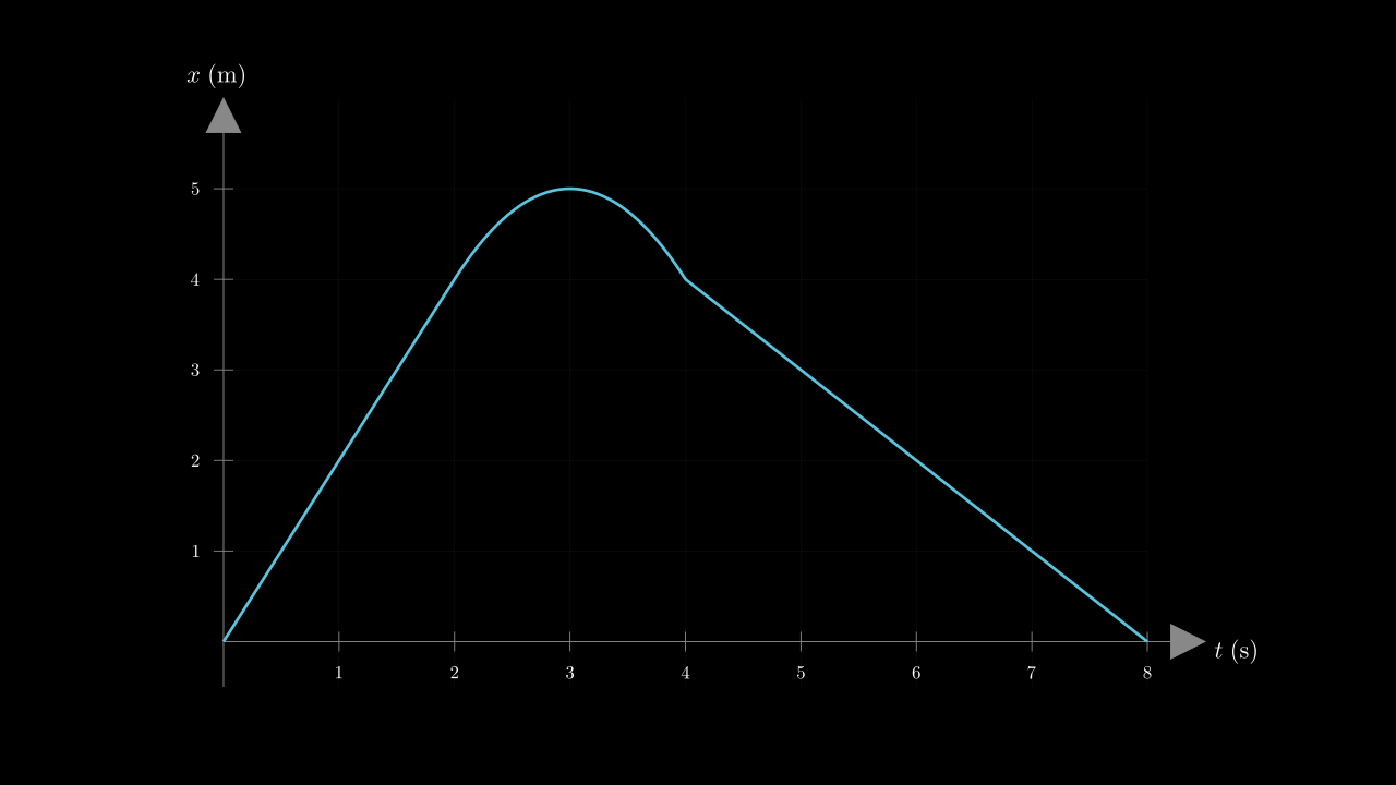
Reading a Graph: What Is the Object Doing?
Look at this position-time graph:
[Image: A position-time graph showing four distinct phases. Phase I ($0 < t < 2\,\text{s}$): a steep, roughly linear rise. Phase II ($2\,\text{s} < t < 4\,\text{s}$): a flat, horizontal section. Phase III ($4\,\text{s} < t < 6\,\text{s}$): a gentle downward curve. Phase IV ($6\,\text{s} < t < 8\,\text{s}$): a steep downward curve. The phases are labeled I through IV directly on the graph.]
Prediction: For each phase, describe what the object is doing physically. Where is it fast? Where is it slow? Where does it change direction? Commit to your answers before continuing.
Here is what each phase tells us:
-
Phase I -- Steep upward slope. The object is moving in the positive direction at a relatively high, roughly constant velocity. Steep slope on an $x(t)$ graph means large $\frac{dx}{dt}$, which means fast.
-
Phase II -- Flat (horizontal) section. The position is not changing. The object is at rest. Slope is zero, so $v = 0$.
-
Phase III -- Gentle downward curve. The object has started moving in the negative direction, slowly at first but speeding up. The slope is negative and getting more negative -- the object is accelerating in the negative direction.
-
Phase IV -- Steep downward curve. The object is now moving quickly in the negative direction.
Notice what you just did. You never touched an equation. You read the slope of the graph -- its steepness and sign -- and translated that directly into physical behavior. The graph told a story, and you interpreted it.
This is a skill you will use constantly in mechanics. The position graph encodes everything: velocity lives in the slope, and acceleration lives in the curvature.
The Guiding Question
How can different representations tell the same motion story, and where can they mislead us?
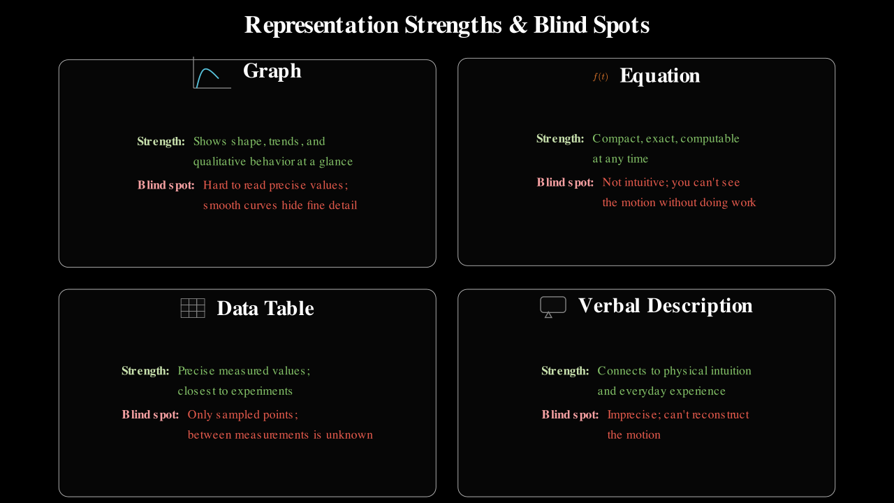
Each representation has strengths and blind spots:
| Representation | Strength | Blind Spot |
|---|---|---|
| Graph | Shows overall shape, trends, and qualitative behavior at a glance | Hard to read precise numerical values; smooth curves can hide fine detail |
| Equation | Compact, exact, and computable at any time | Not intuitive -- you can't "see" the motion without doing work |
| Data table | Gives precise measured values; closest to what experiments produce | Only shows sampled points -- what happens between measurements is unknown |
| Verbal description | Connects to physical intuition and everyday experience | Imprecise; "the car went fast then slowed down" is not enough to reconstruct the motion |
Fluency in mechanics means moving freely among all four. When you get stuck in one representation, switch to another. The insight you need is often hiding in the view you have not tried yet.
Exploration: Translating Between Representations
Graph to Graph: From $x(t)$ to $v(t)$
The key translation rules from $x(t)$ to $v(t)$:
- Where $x(t)$ has a steep positive slope, $v(t)$ is large and positive.
- Where $x(t)$ is flat, $v(t)$ is zero.
- Where $x(t)$ has a negative slope, $v(t)$ is negative.
- Where $x(t)$ has a local maximum or minimum, $v(t)$ crosses zero.
- Where $x(t)$ is curved (concave up or down), $v(t)$ is changing -- meaning there is acceleration.
These are not rules to memorize. They follow directly from the single fact that $v(t) = \frac{dx}{dt}$: velocity is the slope of the position graph.
Watch this process in action. The animation below sweeps across a position graph, reads its slope at every moment, and plots the resulting velocity below.
Graph to Graph: From $v(t)$ to $a(t)$
The same logic applies one level deeper. Acceleration is the slope of the velocity graph, since $a(t) = \frac{dv}{dt}$.
Equation to Graph and Back
Explore how position, velocity, and acceleration relate by adjusting the coefficients in the interactive tool below. The blue curve is $x(t)$, green is $v(t)$, and red is $a(t)$. A gold tangent line shows the slope of $x(t)$ at the current time.
Guided prompts: - Set a flat position (zero velocity and acceleration). What do all three curves look like? - Make the initial velocity positive and half-acceleration negative. At what time does the object stop? How can you tell from each curve? - Can you find settings where velocity is always positive but acceleration changes sign?
MathBox Visualization
Spend time with this tool. Try your own functions. The goal is not to memorize specific curves but to build the reflex: given any one representation, you can construct the others.
Concept Reveal: Fluency Is the Goal
Here is the core idea of this section:
Being good at mechanics does not mean memorizing which formula to use. It means being able to move freely among graphs, equations, data, and physical descriptions -- extracting meaning from each and checking one against the others.
Each representation reveals something the others hide:
- The graph reveals overall shape and qualitative behavior. You can see at a glance where the object speeds up, slows down, or reverses.
- The equation reveals exact values and enables computation. You can plug in any time and get a precise answer.
- The data table reveals what an actual measurement looks like. Real physics comes in tables, not equations -- and those tables are always incomplete.
- The verbal description reveals physical meaning. "The ball rises, slows, stops, and falls" conveys the story in a way no formula can.
When you combine representations, you get something more powerful than any single one. And when two representations seem to disagree, one of them contains an error -- finding that error is one of the deepest things you can practice.
Connection: The Whole Chapter in One View
This section pulls together everything from Chapter 1. Here is how the pieces fit:
- Section 1.1 (Models and idealization): We choose what to model and what to ignore. The representations in this section describe the model, not the full messy reality.
- Section 1.2 (Position function): $x(t)$ is the foundation. Every graph, table, and equation in this section starts from a position function.
- Section 1.3 (Reference frames and coordinates): The numbers in our graphs and tables depend on the coordinate system we chose. A different choice of origin shifts the graph vertically but does not change the physics.
- Section 1.4 (Displacement and path length): Reading displacement from a graph means looking at the vertical difference between two points. Path length requires more -- you need to account for any backtracking.
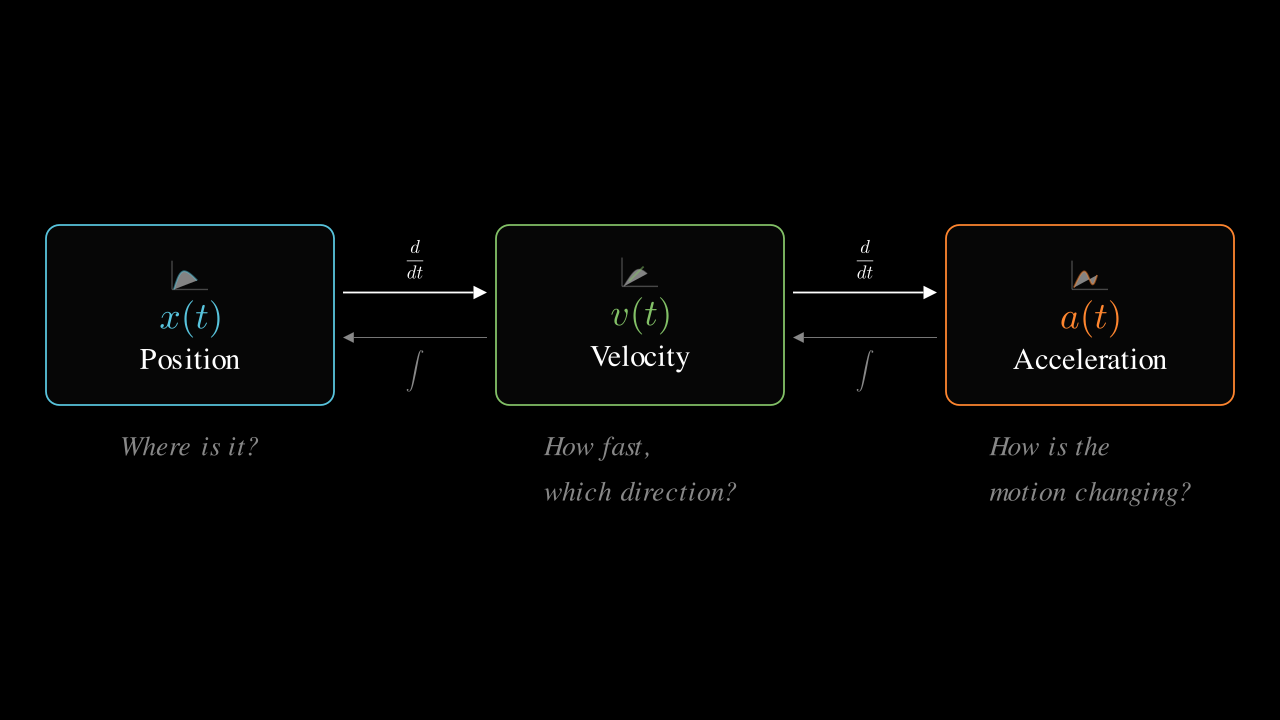
- Section 1.5 (Velocity): Velocity is the slope of $x(t)$. Every time you read a slope from the position graph, you are using the derivative $v = \frac{dx}{dt}$.
- Section 1.6 (Acceleration): Acceleration is the slope of $v(t)$, or equivalently the curvature of $x(t)$. The chain of derivatives -- $x(t) \to v(t) \to a(t)$ -- is the backbone of kinematics.
One function, two derivatives, three levels of description. That is the mathematical structure of motion.
Spaced Retrieval
Before moving to practice, test your memory of earlier material. Try to answer from recall, not by scrolling back.
Recall prompt 1: What is the difference between displacement and path length? Can displacement ever be larger than path length?
Recall prompt 2: A car drives at constant speed around a circular track. Is it accelerating? Why or why not?
Recall prompt 3: You switch from a coordinate system where the origin is at the door to one where the origin is at the window, 3 meters away. What changes about $x(t)$? What stays the same about $v(t)$?
Practice Layers
Layer 1: Concrete -- Read Values
Problem 1. The following table shows position data for a moving cart:
| $t$ (s) | $x$ (m) |
|---|---|
| 0 | 2.0 |
| 1 | 5.0 |
| 2 | 6.0 |
| 3 | 6.0 |
| 4 | 4.0 |
(a) What is the displacement between $t = 0$ and $t = 4\,\text{s}$?
(b) Estimate the average velocity between $t = 0$ and $t = 2\,\text{s}$.
(c) During which time interval is the cart at rest?
(d) During which time interval is the cart moving in the negative direction?
Layer 2: Pattern -- Sketch Derived Graphs
Problem 2. Below is a position-time graph.
(a) Sketch the corresponding $v(t)$ graph. Label the sign and approximate value of velocity in each region.
(b) Sketch the corresponding $a(t)$ graph. Where is acceleration zero? Where is it nonzero?
(c) At what time(s) does the object change direction? How do you know from the $x(t)$ graph? How would you know from the $v(t)$ graph?
Layer 3: Structure -- Reasoning About Incomplete Information
Problem 3. A student collects noisy position data from a sensor. They have 10 measurements, one per second, but each measurement has an uncertainty of $\pm 0.5\,\text{m}$.
(a) Can the student reliably estimate the average velocity over the full 10-second interval? Why or why not?
(b) Can the student reliably estimate the instantaneous velocity at $t = 5\,\text{s}$? What makes this harder than part (a)?
(c) Can the student say anything reliable about the acceleration? What are the limits of what noisy data can tell us?
The lesson here: Differentiation amplifies noise. Average quantities computed over long intervals are robust. Instantaneous quantities estimated from discrete, noisy data are fragile. This is a fundamental tension in experimental physics.
The following animation demonstrates this principle visually -- watch how small measurement errors in position become large errors in velocity, and explode when estimating acceleration.
Layer 4: Debug -- Find the Error
Problem 4. A student is given the position function $x(t) = t^3 - 6t^2 + 9t$ (with $x$ in meters and $t$ in seconds). They produce the following velocity-time graph:
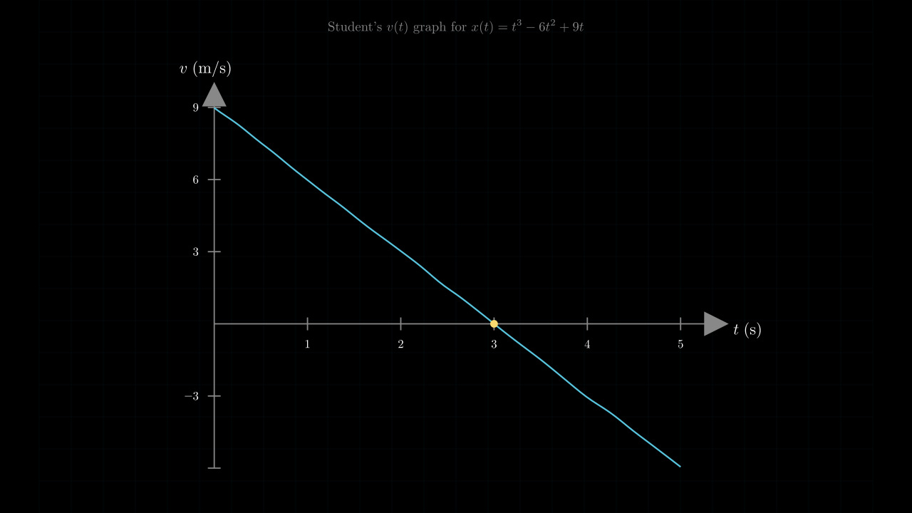
(a) Compute $v(t) = \frac{dx}{dt}$ from the given equation.
(b) Is the student's graph correct? If not, what specific feature is wrong?
(c) What misconception might have led to the student's graph? What did they likely do instead of taking the derivative correctly?
Use the interactive tool below to explore the correct behavior of $x(t) = t^3 - 6t^2 + 9t$ and its derivatives:
MathBox Visualization
Layer 5: Creation -- Design a Motion
Problem 5.
(a) Design a motion -- as an equation or a graph -- where the velocity is always positive but the acceleration changes sign. Describe in words what this motion looks like physically.
(b) Design a motion where the object returns to its starting position at $t = 4\,\text{s}$ but is never at rest during the interval $0 < t < 4\,\text{s}$. Is this possible? If so, provide an example. If not, explain why.
Metacognition
Self-check: This section asked you to translate between four representations -- graphs, equations, data tables, and verbal descriptions. That means there are many possible translations:
- Graph to equation
- Equation to graph
- Data to graph
- Graph to verbal description
- Equation to verbal description
- Data to equation
Which of these translations is hardest for you? That is the one worth practicing most. Go back to the Representation Translator interactive and spend extra time on that specific direction.
Confidence check: Rate yourself (1 to 5) on each of these skills: - I can look at an $x(t)$ graph and describe the velocity qualitatively. - I can look at a $v(t)$ graph and sketch the corresponding $x(t)$ graph. - Given an equation for $x(t)$, I can compute and graph $v(t)$ and $a(t)$. - I can extract motion information from a data table with missing values.
Any score below 3 is a signal, not a failure. It tells you exactly where to focus.
Chapter 1 Summary
This chapter introduced the mathematical language of motion. Here is what we built, piece by piece:
-
Models and idealization (1.1): Real motion is messy. Physics begins by choosing what to keep and what to ignore. The particle model is a deliberate simplification, not a lazy one.
-
Position as a function of time (1.2): The position function $x(t)$ is a complete instruction set for one-dimensional motion. Given $x(t)$, you can answer any question about where the object is at any time.
-
Reference frames and coordinates (1.3): The numbers in $x(t)$ depend on who is watching and how they label positions. The physics does not.
-
Displacement and path length (1.4): Displacement $\Delta x = x(t_2) - x(t_1)$ tells you where you ended up relative to where you started. Path length tells you how much ground you covered. They are different quantities that answer different questions.
-
Velocity (1.5): Velocity is the derivative of position: $v(t) = \frac{dx}{dt}$. It is the slope of the position-time graph, the rate of change of position, and the instantaneous version of "how fast and in what direction."
-
Acceleration (1.6): Acceleration is the derivative of velocity: $a(t) = \frac{dv}{dt} = \frac{d^2 x}{dt^2}$. It measures how velocity is changing -- not how fast the object is going, but how fast the "how fast" is changing.
-
Multiple representations (1.7): The same motion can be described as a graph, an equation, a data table, or a verbal narrative. Fluency means translating freely among all of them.
The single most important idea in this chapter:
$$x(t) \xrightarrow{\frac{d}{dt}} v(t) \xrightarrow{\frac{d}{dt}} a(t)$$
One function. Two derivatives. The complete kinematic description of one-dimensional motion.
Chapter-End Retrieval
Close your notes. Put away the scrollbar. Answer these from memory.
1. What is the relationship between position, velocity, and acceleration? How does calculus connect them?
2. What is the difference between displacement and path length? Give an example where they are very different.
3. A position-time graph is flat for a while, then curves upward. Describe the velocity and acceleration during each phase.
4. Why does differentiating noisy data amplify the noise? What does this mean for extracting velocity from measured position data?
5. In one sentence, summarize the big idea of Chapter 1.
After you have attempted all five, check your answers against the chapter summary above.
Reflection
Final thought: You started this chapter with an intuitive sense of motion -- things move, speed up, slow down, turn around. You now have a precise mathematical framework for all of it. A single function $x(t)$ and the operation of differentiation give you velocity and acceleration. Graphs, equations, data, and words are four windows into the same reality.
What did this chapter actually teach you? Write one sentence. Not a sentence about what was covered -- a sentence about what you understand now that you did not understand before.