1.5 Velocity as the Derivative of Position

The speed camera and the GPS

A speed camera catches you at one instant. It fires a radar pulse, measures the Doppler shift, and prints a number: 72 km/h. Done. One moment, one measurement.

Your GPS, meanwhile, records your position every second. It knows where you were at 2:14:03 and where you were at 2:14:04. From those two positions, it computes a speed. But that speed is an average over the one-second gap. If you were braking hard during that second, the GPS number doesn't capture the full story.

So which device is telling the truth about your motion right now? The speed camera, somehow, gets at the instantaneous value. The GPS gets an average. The deep question of this section is: how does the instantaneous value emerge from averages? And the answer turns out to be the single most important idea connecting calculus to physics.

Prediction

Before we work through the math, let's build some intuition.

[Interactive: Predict-then-reveal. Display a curved position-vs-time graph $x(t)$ with a clearly marked point at time $t_0$. The curve should rise, flatten, then dip, so the marked point sits near the flat region. Ask the student to commit to an answer before revealing.]

Look at this position-vs-time graph. At the marked time $t_0$, is the velocity positive, negative, or zero?

Commit to your answer before continuing.

After you commit, a tangent line appears at the marked point. The slope of that tangent line is the velocity. If the slope tilts upward, velocity is positive. If it tilts downward, velocity is negative. If the tangent line is horizontal, velocity is zero.

You just did something important: you read velocity from a position graph, without computing anything. The slope of the position curve tells you how fast and in what direction the object is moving. The rest of this section makes that idea precise.

From average velocity to instantaneous velocity

What you already know

In Section 1.4, we defined displacement as the change in position: $\Delta x = x(t_2) - x(t_1)$. If you divide displacement by the time interval $\Delta t = t_2 - t_1$, you get the average velocity over that interval:

$$\bar{v} = \frac{\Delta x}{\Delta t} = \frac{x(t_2) - x(t_1)}{t_2 - t_1}$$

This is a number you can compute from any two data points. It tells you the overall rate of position change between $t_1$ and $t_2$.

Graphically, this average velocity is the slope of the secant line connecting the two points $(t_1, x(t_1))$ and $(t_2, x(t_2))$ on the position-time graph.

But average velocity hides details. If a runner sprints the first half of a race and walks the second half, the average velocity over the full race doesn't capture either phase. To understand the motion at a specific moment, we need something sharper.

The limit process: shrinking the interval

Here's the key move. Instead of computing the average velocity over a large interval, compute it over a smaller one. Then a smaller one still. Watch what happens.

[Interactive: Drag-to-limit exploration. A smooth, curved position-time graph is displayed with two draggable points on it. A secant line connects the two points, and a readout shows the average velocity (the slope of the secant). The student drags the second point closer to the first, watching the secant line rotate and the average velocity value update in real time.]

Drag the second point toward the first. Watch the secant line and the average velocity value as you do.

• What happens to the slope of the secant line as the two points get closer together?
• Does the average velocity value jump around wildly, or does it settle toward a specific number?
• At what point does the value stop changing meaningfully?

As the interval shrinks, the secant line rotates toward a limiting position: the tangent line at the first point. The average velocity converges to a single, stable value. That stable value is the instantaneous velocity at that moment.

This is the limit process from calculus, applied to a physical situation. You just watched it happen.

A numerical view

To see the convergence concretely, suppose $x(t) = t^2$ (position in meters, time in seconds) and we want the instantaneous velocity at $t = 2$ s.

$t_1$	$t_2$	$\Delta t$	$\Delta x = t_2^2 - t_1^2$	$\bar{v} = \Delta x / \Delta t$
2	3	1	5	5 m/s
2	2.5	0.5	2.25	4.5 m/s
2	2.1	0.1	0.41	4.1 m/s
2	2.01	0.01	0.0401	4.01 m/s
2	2.001	0.001	0.004001	4.001 m/s

The average velocity is converging to 4 m/s. That's the instantaneous velocity at $t = 2$ s.

Notice you never actually reach $\Delta t = 0$ (that would be dividing by zero). You take the limit as $\Delta t$ approaches zero. The value the averages settle toward is the answer.

Concept reveal: velocity is the derivative

What you just computed, through the interactive and the table, has a name in calculus: the derivative.

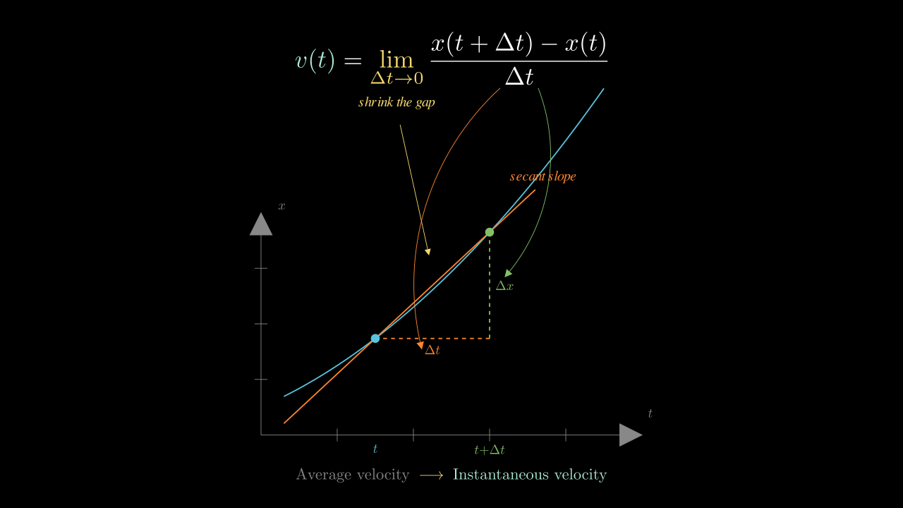
$$v(t) = \frac{dx}{dt} = \lim_{\Delta t \to 0} \frac{x(t + \Delta t) - x(t)}{\Delta t}$$

This is not a new idea layered on top of what you already know. It is what you already know, written in compact notation. The fraction $\frac{\Delta x}{\Delta t}$ is the average velocity. The limit as $\Delta t \to 0$ is the process of shrinking the interval until the value stabilizes. The result, $\frac{dx}{dt}$, is the instantaneous velocity.

Three things to notice:

1. The derivative is a function. You can evaluate $v(t)$ at any time $t$, not just $t = 2$. It gives you the velocity at every moment.

2. The sign matters. If $\frac{dx}{dt} > 0$, position is increasing -- the object moves in the positive direction. If $\frac{dx}{dt} < 0$, position is decreasing -- the object moves in the negative direction. If $\frac{dx}{dt} = 0$, the object is (instantaneously) at rest.

3. Velocity is not speed. Velocity has a sign that indicates direction. Speed is the magnitude: $|\,v(t)\,|$. An object moving to the left at 5 m/s has velocity $-5$ m/s and speed 5 m/s.

Applying it: the power rule in action

For our example $x(t) = t^2$, you can compute the derivative using the power rule from calculus:

$$v(t) = \frac{d}{dt}(t^2) = 2t$$

At $t = 2$ s: $v(2) = 2(2) = 4$ m/s. This matches the value our table converged to. The derivative gives the same answer as the limit process -- because it is the limit process, packaged into a shortcut.

Seeing velocity four ways

A concept understood from one angle is fragile. Let's see velocity from every angle at once.

[Interactive: Four-panel synchronized display. All four panels show the same motion simultaneously and update together in real time.

• Panel 1 (top-left): The $x(t)$ graph with a movable marker. A tangent line at the marker shows the slope.
• Panel 2 (top-right): The $v(t)$ graph. A dot on this graph corresponds to the marker's position on the $x(t)$ graph, showing the velocity value at that moment.
• Panel 3 (bottom-left): A number line with an animated dot moving according to $x(t)$. The dot's speed and direction correspond to the velocity.
• Panel 4 (bottom-right): A live numerical readout: "Position: ___ m, Velocity: ___ m/s."

The student drags the time marker and watches all four panels respond.]

Drag the time marker slowly from left to right. As you do, watch all four panels.

• When the $x(t)$ curve slopes upward steeply, what happens to the dot on the number line? What does the $v(t)$ graph show?
• Find a moment where the $x(t)$ curve is flat. What is the velocity there? What is the dot doing?
• Find a moment where the $x(t)$ curve slopes downward. What is the sign of the velocity? Which direction does the dot move?

This is the core skill of kinematics: reading motion across representations. The slope of the position graph, the value on the velocity graph, the behavior of the moving dot, and the numerical readout are all saying the same thing in different languages.

Connection to what you already know

The derivative from your calculus course is not a different concept here. It's the same limit, the same process, the same rules (power rule, chain rule, all of it). What's different is the meaning of the variables:

Calculus class	Physics
$f(x)$	$x(t)$ -- position as a function of time
$x$	$t$ -- time is the independent variable
$f'(x)$	$v(t) = \frac{dx}{dt}$ -- velocity
Slope of the tangent	How fast the object is moving

You already know how to differentiate. Now you know what differentiation means when the function describes motion. Every derivative rule you learned is a tool for extracting velocity from a position function.

Historical note

Newton invented calculus precisely because he needed instantaneous rates of change to describe planetary motion. He wanted to know not just where a planet was at two different times, but how fast and in what direction it was moving at each instant. The limit process -- shrinking $\Delta t$ toward zero -- was his answer.

You're now using his tool for exactly its original purpose. The derivative wasn't a pure math invention that physics borrowed later. Physics demanded it, and calculus was built to meet that demand.

Spaced recall

Before we move to practice, a quick check on earlier material.

From Section 1.4: What is the difference between displacement and path length? Can displacement ever exceed path length?

Take a moment to recall your answer before moving on. If you're unsure, revisit Section 1.4 -- this distinction will keep coming back.

Practice layers

Layer 1: Concrete computation

Problem 1. A particle's position is given by $x(t) = 3t^2 - 2t + 1$ (meters, seconds).

(a) Compute the average velocity between $t = 1$ s and $t = 3$ s.

(b) Find the instantaneous velocity $v(t)$ by differentiating.

(c) Evaluate $v(1)$ and $v(3)$. How do these compare to the average velocity from part (a)?

Problem 2. A car's position is $x(t) = 5t - t^2$ for $0 \leq t \leq 5$ s.

(a) At what time is the velocity zero?

(b) Is the car moving to the right or to the left at $t = 1$ s? At $t = 4$ s?

(c) What is the car's speed at $t = 4$ s? (Careful: speed is not the same as velocity.)

Layer 2: Pattern -- reading $v(t)$ to sketch $x(t)$

[Interactive: A $v(t)$ graph is shown (piecewise: positive constant, then zero, then negative constant). The student sketches what $x(t)$ might look like on a blank set of axes. After submitting their sketch, the correct $x(t)$ graph overlays for comparison.]

Given this velocity-vs-time graph, sketch the position-vs-time graph. Think about what each segment of $v(t)$ means for how position is changing.

Hints to guide your thinking: - When $v > 0$, position is _ (increasing/decreasing). - When $v = 0$, position is _. - When $v < 0$, position is _. - Constant velocity means the position graph is a _ line.

Layer 3: Structural reasoning

Can an object have zero velocity but nonzero position?

Think of a concrete example. A ball thrown straight up, at the very top of its arc: its position is far from zero (it's high in the air), but for one instant, its velocity is exactly zero.

Position and velocity are independent quantities. Position tells you where something is. Velocity tells you how that position is changing. Knowing one does not determine the other.

Can an object have zero position but nonzero velocity?

Again, think concretely. A car passes through the origin ($x = 0$) at full speed. At that instant, $x = 0$ but $v \neq 0$. Position zero doesn't mean the object has stopped -- it means the object happens to be at the origin.

Layer 4: Debug

A student says: "The object is at $x = 5$ m, so it must be moving to the right."

What's wrong with this reasoning?

The student is confusing position with velocity. Position tells you where the object is, not which way it's going. An object at $x = 5$ m could be: - moving to the right ($v > 0$), - moving to the left ($v < 0$), - momentarily at rest ($v = 0$).

To determine direction, you need the velocity -- the derivative of position -- not the position itself. This is one of the most common errors in introductory mechanics: reading motion information from a quantity that only encodes location.

Layer 5: Transfer

The relationship between a quantity and its rate of change isn't unique to motion. Consider a bank account.

Let $B(t)$ be your bank balance as a function of time (in days). Then $\frac{dB}{dt}$ is the rate at which money is entering or leaving the account.

If $\frac{dB}{dt} > 0$, deposits exceed withdrawals -- your balance is growing.

If $\frac{dB}{dt} < 0$, withdrawals exceed deposits -- your balance is shrinking.

If $\frac{dB}{dt} = 0$, the balance is momentarily constant.

The math is identical to position and velocity. The derivative of a quantity tells you how fast and in what direction that quantity is changing. "Position" and "velocity" are just the names we give these ideas when the quantity is location and the independent variable is time.

Exercise: Your bank balance follows $B(t) = 1000 + 50t - 2t^2$ (dollars, where $t$ is in weeks).

(a) Find $\frac{dB}{dt}$.

(b) At what time is the balance at its maximum?

(c) Is your balance growing or shrinking at $t = 20$ weeks?

Key ideas summary

Let's collect the essential points from this section.

Average velocity is the slope of the secant line on a position-time graph:

$$\bar{v} = \frac{x(t_2) - x(t_1)}{t_2 - t_1}$$

Instantaneous velocity is the slope of the tangent line -- the limit of average velocity as the interval shrinks to zero:

$$v(t) = \frac{dx}{dt} = \lim_{\Delta t \to 0} \frac{x(t + \Delta t) - x(t)}{\Delta t}$$

Sign and direction: $v > 0$ means motion in the positive direction; $v < 0$ means motion in the negative direction; $v = 0$ means instantaneously at rest.

Velocity vs. speed: Velocity has a sign (direction). Speed is $|v|$ (magnitude only).

Position does not determine velocity. Knowing where an object is tells you nothing about how it's moving. You need the derivative for that.

Reflection

In your own words, what is the relationship between the position graph and the velocity graph?

Take a moment to write or say your answer before reading on.

Here is one way to think about it: the velocity graph is a commentary on the position graph. Wherever the position graph is rising, the velocity graph is positive. Wherever the position graph is falling, the velocity graph is negative. Wherever the position graph levels off, the velocity graph crosses zero. The steeper the position graph, the larger the velocity. The velocity graph doesn't tell you where the object is -- it tells you what the position graph is doing.

In the next section, we'll push this idea one level deeper: what happens when you take the derivative of velocity?